
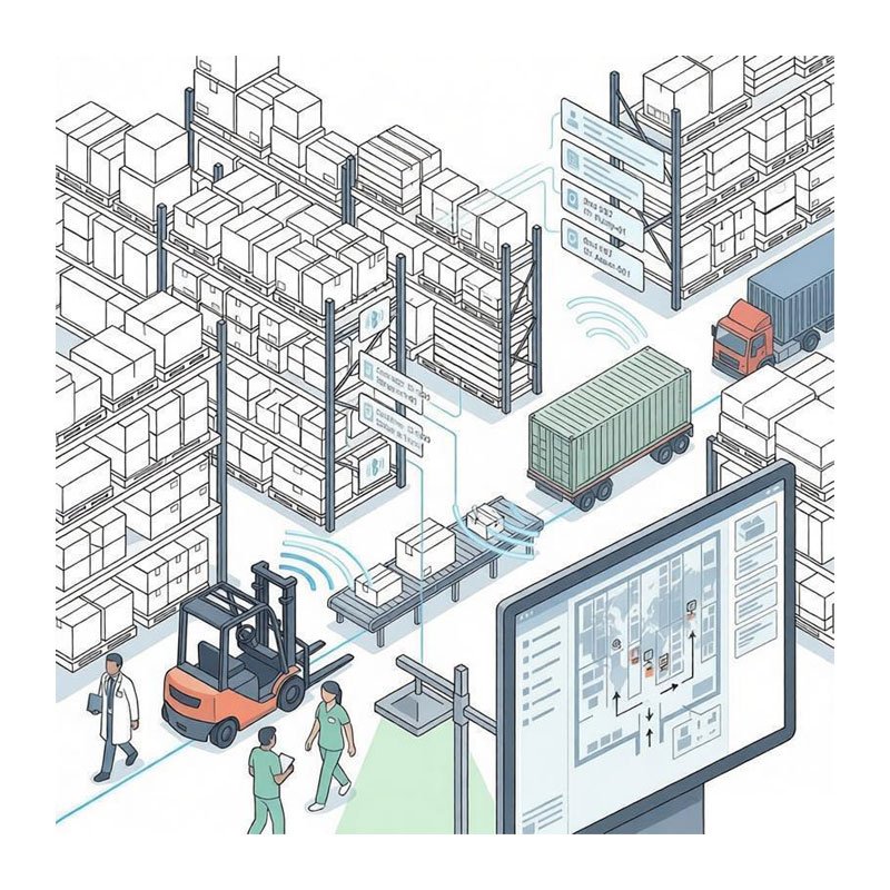
Building a BLE tag asset tracking system is not about choosing the right tag. It is about the infrastructure that receives, filters, transports, and stores the data from hundreds or thousands of tags scattered across a facility. The tag itself is a dumb broadcaster; the intelligence lives in the gateway network, the edge processor, and the cloud backend. This article breaks down the full system architecture from radio reception to dashboard, with hardware selection tables, filtering algorithms, data pipeline schemas, and deployment cost models drawn from production deployments in hospitals, warehouses, and manufacturing floors.
1. System Architecture Overview
A production BLE asset tracking system has four tiers, each with distinct latency, throughput, and reliability requirements:
| Tier | Components | Latency Budget | Data Volume | Failure Impact |
|---|---|---|---|---|
| T1: Tag Layer | BLE tags (hundreds to thousands) | N/A (broadcast only) | ~30 bytes/tag/event | Single asset goes dark |
| T2: Gateway Layer | BLE scanners (5-50 units) | 100-500 ms scan cycle | ~50 KB/s peak per gateway | Zone goes dark (10-50 tags) |
| T3: Edge Layer | Local server or edge appliance | 1-5 s processing | ~200 KB/s aggregated | Tracking delayed, not lost |
| T4: Cloud Layer | Backend, database, dashboard | 1-10 s end-to-end | ~500 KB/s sustained | Historical data gap |
The most common architecture mistake is treating the gateway as a simple relay that forwards raw BLE packets to the cloud. At 500 tags with 1-second advertising intervals and 10 gateways, that is 5,000 packets per second hitting your cloud ingest endpoint, each containing duplicate RSSI readings from overlapping coverage zones. Edge filtering is not an optimization; it is a requirement.
2. Gateway Hardware Selection
The gateway is the most critical hardware decision in the system. It must simultaneously scan BLE advertising channels, run filtering logic, maintain network connectivity, and survive power disruptions. Three hardware families dominate production deployments:
| Platform | BLE Chip | CPU | RAM | Power | Cost (BOM) | Best For |
|---|---|---|---|---|---|---|
| ESP32-Based | ESP32 (dual-mode) | 240 MHz Xtensa x2 | 520 KB SRAM | 2.5W (WiFi+BLE) | $3-5 | Small sites, WiFi backhaul |
| Raspberry Pi + USB Dongle | nRF52840 dongle | 1.4 GHz ARM Cortex-A72 x4 | 1-4 GB | 5-7W | $45-60 | R&D, prototyping, low-volume |
| Purpose-Built Gateway | nRF52832/52840 + ESP32 | ESP32 240MHz + nRF52 | 520KB + 256KB | 2-3W | $15-25 | Production deployments |
| Industrial Gateway (Linux) | CC2640R2 + WiFi/LTE | ARM Cortex-A7 1GHz | 512 MB | 5-15W | $200-400 | Harsh environments, cellular |
2.1 ESP32 as a Gateway: Capabilities and Limits
The ESP32 is the most common gateway platform for cost-sensitive deployments because it has built-in WiFi and BLE. However, the ESP32 BLE controller shares the 2.4 GHz radio between WiFi and BLE, meaning it cannot scan BLE while transmitting WiFi. This time-division multiplexing introduces scan gaps:
| WiFi Activity | BLE Scan Gap | Packet Loss (1s interval) | Packet Loss (500ms) |
|---|---|---|---|
| Idle (beacon only) | 0 ms | 0% | 0% |
| MQTT publish (every 5s) | ~15 ms/gap | 0.3% | 0.6% |
| WiFi streaming (continuous) | ~50 ms/gap | 1.0% | 2.0% |
| OTA update | ~200 ms/gap | 5-8% | 10-15% |
For a hospital tracking 200 tags with 1-second intervals, a 1% loss rate means 2 tags missing per scan cycle. This is tolerable for presence detection but problematic for real-time RTLS. The solution is either a dual-radio gateway (ESP32 for WiFi + nRF52 for BLE) or reducing WiFi activity to periodic batch uploads.
2.2 Purpose-Built Gateway Architecture
Production gateways typically pair an nRF52 (dedicated BLE scanner) with an ESP32 (WiFi/CPU). The nRF52 runs continuous active scan and forwards packets over UART/SPI to the ESP32, which handles filtering, buffering, and cloud communication. This dual-chip design eliminates radio contention entirely.
# Gateway firmware data flow (nRF52 + ESP32)

# nRF52 side: continuous BLE scanner
def ble_scan_callback(adv_report):
packet = {
"mac": adv_report.peer_addr,
"rssi": adv_report.rssi,
"adv_type": adv_report.type,
"data": adv_report.data,
"ts": get_timestamp_us(),
}
uart_send(json.dumps(packet))  # ~120 bytes/packet

# ESP32 side: receive, filter, batch upload
rx_buffer = []
def uart_rx_callback(data):
pkt = json.loads(data)
if should_forward(pkt):  # edge filtering
rx_buffer.append(pkt)
if len(rx_buffer) >= BATCH_SIZE or time_since_last_upload > UPLOAD_INTERVAL:
upload_batch(rx_buffer)
rx_buffer.clear()
2.3 Gateway Placement and Coverage
Gateway density is the single largest cost driver. Too few gateways leave coverage holes; too many create redundant data and unnecessary filtering load. The optimal density depends on the required location accuracy and the physical environment:
| Accuracy Tier | Gateways per 100 m2 | Typical Spacing | Cost per m2 | Use Case |
|---|---|---|---|---|
| Presence (room-level) | 0.5-1.0 | 10-15 m | $0.15-0.30 | Asset presence per zone |
| Coarse positioning (3-5 m) | 2-4 | 5-8 m | $0.60-1.20 | Warehouse aisle tracking |
| Fine positioning (1-2 m) | 6-10 | 3-5 m | $1.80-3.00 | Surgical instrument tracking |
| Sub-meter (0.5 m) | 15-25 | 2-3 m | $4.50-7.50 | High-value asset audit |
These numbers assume open-plan environments. Walls, metal shelving, and equipment racks reduce effective range by 30-50%. A warehouse with 8 m steel racks may need 2x the gateway density of an open hospital corridor for the same accuracy.
3. BLE Scanning Strategy
The gateway must decide how to scan BLE advertising channels. The BLE spec defines three advertising channels (37, 38, 39) that tags hop across. A scanner can either listen on one channel or cycle through all three. The scan window and interval parameters control how much time the radio spends listening versus sleeping.
3.1 Active vs. Passive Scan
| Parameter | Passive Scan | Active Scan |
|---|---|---|
| Sends SCAN_REQ | No | Yes |
| Receives SCAN_RSP | No | Yes (up to 31 bytes extra) |
| Power consumption | Lower (Rx only) | Higher (Tx + Rx) |
| Tag power impact | None | +20-40% if tag responds to all scans |
| Data available | 31 bytes (adv packet only) | 62 bytes (adv + scan response) |
| Latency to first detection | ~1 adv interval | ~1 adv interval |
For asset tracking with custom payloads in the manufacturer-specific data, passive scan is sufficient. Active scan is necessary only when the tag splits data between the advertising packet and scan response (e.g., iBeacon UUID in adv + sensor data in scan response).
3.2 Scan Window and Interval
The scan interval defines how often the scanner starts a scan cycle. The scan window defines how long each cycle lasts. If window equals interval, the scanner runs continuously (100% duty cycle). Production gateways typically use 80-100% duty cycle because the power budget is not battery-constrained.
| Scan Interval | Scan Window | Duty Cycle | Capture Rate (1s tag interval) | Capture Rate (500ms) |
|---|---|---|---|---|
| Continuous | Continuous | 100% | ~99.5% | ~99.0% |
| 1000 ms | 1000 ms | 100% | ~99.5% | ~99.0% |
| 1000 ms | 500 ms | 50% | ~50-65% | ~50-65% |
| 2000 ms | 1000 ms | 50% | ~50-65% | ~50-65% |
| 5000 ms | 1000 ms | 20% | ~20-30% | ~20-30% |
The capture rate at 50% duty cycle is not exactly 50% because of the probabilistic overlap between the scan window and the tag’s advertising events. With three advertising channels and random phase, the actual capture rate follows a birthday-problem distribution. For production deployments, continuous scan (100% duty cycle) is strongly recommended unless the gateway is battery-powered.
3.3 Duplicate Filtering at the Radio Level
The BLE controller reports each advertising packet it receives, including duplicates from the same tag within the same scan window. A tag advertising at 100 ms generates 10 packets per second per gateway. With 500 tags and 10 gateways, that is 50,000 packets per second across the system. The controller can optionally suppress duplicates:
| Filter Mode | Duplicates Reported | Packets/s (500 tags, 1s, 10 GW) | Gateway CPU Load |
|---|---|---|---|
| No filtering | All | ~15,000 | High |
| Controller-level dedup (per scan cycle) | 1 per tag per cycle | ~500 | Low |
| Application-level dedup (sliding window) | 1 per tag per window | ~500 | Low-Medium |
The nRF52 BLE API supports duplicate filtering via sd_ble_gap_scan_start() with scan_params.filter_policy set to BLE_GAP_SCAN_FP_DUPLICATE. This reduces the interrupt load dramatically but means the application only gets one RSSI sample per tag per scan cycle (typically 1 second).
4. Edge Filtering: Reducing Data Before the Cloud
Even with radio-level dedup, overlapping gateway coverage means the same tag is reported by multiple gateways. Edge filtering is the process of selecting the best report and discarding the rest. This typically happens on the edge server (T3) or a designated gateway acting as an aggregator.
4.1 Multi-Gateway Deduplication
When 3 gateways report the same tag within a 1-second window, only one record should reach the cloud. The selection algorithm must consider RSSI, timestamp, and gateway reliability:
# Edge deduplication algorithm
DEDUP_WINDOW_MS = 2000  # 2-second sliding window

def deduplicate(raw_reports):
# Select best report per tag within dedup window
by_tag = group_by_mac(raw_reports)
result = []
for mac, reports in by_tag.items():
if len(reports) == 1:
result.append(reports[0])
continue
# Score each report: weighted RSSI + freshness + reliability
best = max(reports, key=lambda r: score_report(r))
result.append(best)
return result

def score_report(r):
# RSSI: higher is better (closer), normalize -100 to -30
rssi_score = (r.rssi + 100) / 70  # 0.0 to 1.0
# Freshness: newer is better, penalize >5s old
age_s = (now() - r.ts) / 1000
fresh_score = max(0, 1 - age_s / 5)
# Reliability: weighted by gateway uptime percentage
gw_reliability = gateway_stats[r.gw_id].uptime_pct
return rssi_score * 0.6 + fresh_score * 0.2 + gw_reliability * 0.2
4.2 RSSI Smoothing and Outlier Rejection
Raw RSSI from a single packet is noisy. Multipath reflections, body absorption, and interference cause +/-10 dB swings. For location estimation, the edge should apply smoothing before forwarding:
| Filter | Window Size | Latency Added | RSSI Variance Reduction | Implementation Complexity |
|---|---|---|---|---|
| Raw (no filter) | 1 sample | 0 s | 0% | None |
| Moving average | 5 samples | 2-5 s | ~55% | Low (FIFO buffer) |
| Exponential smoothing | Infinite (weighted) | 1-3 s | ~50% | Low (1 multiply) |
| Median filter | 3-7 samples | 1-3 s | ~65% | Medium (sort) |
| Kalman filter | Adaptive | 0.5-2 s | ~70% | High (matrix math) |
Exponential smoothing (alpha = 0.3) is the production default for most deployments because it requires only one previous value and one multiply:
# Exponential RSSI smoothing (alpha = 0.3)
# New value = alpha * raw + (1 - alpha) * previous
ALPHA = 0.3
smoothed_rssi = {}

def smooth_rssi(mac, raw_rssi):
if mac not in smoothed_rssi:
smoothed_rssi[mac] = raw_rssi
else:
smoothed_rssi[mac] = ALPHA * raw_rssi + (1 - ALPHA) * smoothed_rssi[mac]
return round(smoothed_rssi[mac], 1)
4.3 Event-Based Forwarding
Instead of forwarding every scan cycle, the edge can forward only when meaningful events occur. This reduces cloud traffic by 80-95% while preserving tracking accuracy:
| Forwarding Strategy | Packets/Tag/Hour | Cloud BW (500 tags) | Use Case |
|---|---|---|---|
| Every scan (1s) | 3,600 | ~14 MB/h | RTLS with sub-second updates |
| Every 5s (batch) | 720 | ~2.8 MB/h | Standard tracking |
| Zone change only | ~5-20 | ~40 KB/h | Room-level presence |
| Threshold breach + heartbeat | ~2-10 | ~20 KB/h | Temperature/humidity alerts |
5. Data Pipeline Design
The data pipeline transports filtered tag data from the edge to the cloud backend. Three transport protocols are commonly used, each with different reliability, latency, and complexity tradeoffs:
5.1 Transport Protocol Comparison
| Protocol | Overhead/Packet | Reliability | Latency | Power (Gateway) | Best For |
|---|---|---|---|---|---|
| HTTP POST (JSON) | ~400 bytes (headers) | TCP (guaranteed) | 100-500 ms | High (connection setup) | Small deployments, simple backends |
| MQTT (QoS 1) | ~20 bytes (header) | TCP + ACK | 50-200 ms | Low (persistent connection) | Production deployments |
| UDP (custom) | ~8 bytes (header) | None (best-effort) | 10-50 ms | Lowest | Real-time RTLS, local LAN |
| LoRaWAN (gateway-to-cloud) | ~13 bytes (header) | Confirmed downlink | 1-10 s | N/A | Remote sites without WiFi |
MQTT is the industry default for BLE asset tracking because it maintains a persistent TCP connection (eliminating HTTP connection setup overhead), supports QoS levels for guaranteed delivery, and has a lightweight publish/subscribe model that maps naturally to multi-zone tracking (each zone is a topic).
5.2 MQTT Topic Structure
# MQTT topic hierarchy for asset tracking
# Format: site/zone/gateway/tag/event

site-001/zone-A/gw-01/+/scan      # All scans from gw-01
site-001/zone-A/+/tag-005/scan    # All scans of tag-005 in zone-A
site-001/+/+/tag-005/zone_change  # Zone change events for tag-005
site-001/+/+/+/battery_low         # Battery alerts across site
site-001/+/+/+/temperature_alert   # Temperature threshold breaches

# Payload format (JSON, ~80 bytes)
{
"mac": "AA:BB:CC:DD:EE:01",
"rssi": -67,
"gw": "gw-01",
"ts": 1722422400000,
"bat": 85,
"temp": 23.5,
"seq": 4823
}
5.3 Data Schema and Storage
The cloud backend typically uses a time-series database for raw scan data and a relational database for asset metadata:
| Store | Technology | Data | Retention | Query Pattern |
|---|---|---|---|---|
| Time-series (hot) | InfluxDB / TimescaleDB | Raw scan events | 7-30 days | Range queries by tag + time |
| Time-series (cold) | S3 / Parquet | Aggregated events | 1-5 years | Batch analytics, compliance |
| Relational | PostgreSQL / MySQL | Asset metadata, zones, users | Permanent | CRUD, joins |
| Cache | Redis | Last-known location | TTL 5 min | Sub-ms lookup |
5.4 Storage Sizing
# Storage sizing calculation for 500 tags, 5s forwarding interval
tags = 500
events_per_tag_per_hour = 3600 / 5  # = 720
events_per_hour = tags * events_per_tag_per_hour  # = 360,000
events_per_day = events_per_hour * 24  # = 8,640,000

bytes_per_event = 80  # JSON payload
bytes_per_day = events_per_day * bytes_per_event  # = 691 MB/day
bytes_per_month = bytes_per_day * 30  # = ~20.7 GB/month (raw)
bytes_per_year = bytes_per_day * 365  # = ~252 GB/year (raw)

# With compression (Parquet, ~5:1 ratio):
compressed_per_year = bytes_per_year / 5  # = ~50 GB/year

# Database overhead (indexes, WAL, etc.): +40%
total_storage_year = compressed_per_year * 1.4  # = ~70 GB/year
6. Location Estimation at the Edge
For systems that need more than room-level presence, the edge performs location estimation using RSSI from multiple gateways. The three most common algorithms have different accuracy, complexity, and gateway requirements:
| Algorithm | Min Gateways | Accuracy | Edge CPU | Calibration | Best For |
|---|---|---|---|---|---|
| Proximity (strongest RSSI) | 1 | Room-level (5-10 m) | Minimal | None | Simple presence |
| Weighted centroid | 3+ | 3-5 m | Low | Gateway positions only | Open areas |
| Trilateration (log-distance) | 3+ | 2-4 m | Medium | Path-loss exponent per zone | Warehouses, corridors |
| Fingerprinting (kNN) | 4+ | 1-3 m | Medium-High | Full RF survey (hours) | Complex indoor environments |
| BLE Angle of Arrival (AoA) | 1 (with antenna array) | 0.5-1 m | High | Antenna phase calibration | High-value asset tracking |
6.1 Weighted Centroid Algorithm
The weighted centroid is the production default because it requires no calibration beyond gateway positions and provides 3-5 m accuracy in open areas:
# Weighted centroid location estimation
# Weight = 10^(RSSI/10), giving closer gateways exponentially more weight

def estimate_position(reports, gateway_positions):
# reports: [{"gw_id": "gw-01", "rssi": -65}, ...]
# gateway_positions: {"gw-01": (x, y), ...}
total_weight = 0
weighted_x = 0
weighted_y = 0

for r in reports:
gw_id = r["gw_id"]
if gw_id not in gateway_positions:
continue
# Convert RSSI to weight (closer = higher weight)
weight = 10 ** (r["rssi"] / 10)
gx, gy = gateway_positions[gw_id]
weighted_x += weight * gx
weighted_y += weight * gy
total_weight += weight

if total_weight == 0:
return None

return (weighted_x / total_weight, weighted_y / total_weight)

# Example: tag detected by 3 gateways
reports = [
{"gw_id": "gw-01", "rssi": -55},  # Close (weight = 316)
{"gw_id": "gw-02", "rssi": -75},  # Far (weight = 0.032)
{"gw_id": "gw-03", "rssi": -65},  # Medium (weight = 3.16)
]
positions = {
"gw-01": (10, 20),
"gw-02": (30, 40),
"gw-03": (50, 10),
}
# Result: ~(10.9, 20.1) - heavily weighted toward gw-01
7. System Reliability and Failover
7.1 Gateway Health Monitoring
Each gateway must report health metrics so the edge can detect failures and trigger alerts:
| Metric | Normal Range | Alert Threshold | Check Interval |
|---|---|---|---|
| Packets/minute | 50-500 (depends on tag count) | < 10 or > 2000 | 60 s |
| CPU temperature | 40-65 C | > 75 C | 300 s |
| WiFi RSSI | -30 to -65 dBm | < -75 dBm | 60 s |
| Uptime | > 99.5% | < 99% | Daily |
| Last heartbeat | < 30 s ago | > 120 s ago | 30 s |
7.2 Edge-to-Cloud Connectivity Loss
When the edge loses cloud connectivity (WiFi outage, ISP failure), it must buffer data locally and replay when connectivity returns. The buffer sizing depends on the maximum acceptable downtime:
| Max Downtime | Buffer Size (500 tags, 5s interval) | Storage Medium | RAM vs Disk |
|---|---|---|---|
| 15 min | ~4.3 MB | RAM | In-memory queue |
| 1 hour | ~17 MB | RAM or SD card | In-memory or file |
| 4 hours | ~69 MB | SD card / eMMC | SQLite + WAL |
| 24 hours | ~415 MB | SSD / eMMC | SQLite + compression |
# Edge buffering with SQLite for offline-first operation
import sqlite3, json, time

class EdgeBuffer:
def __init__(self, db_path="/data/edge_buffer.db"):
self.conn = sqlite3.connect(db_path)
self.conn.execute(
"CREATE TABLE IF NOT EXISTS events ("
"id INTEGER PRIMARY KEY AUTOINCREMENT, "
"ts INTEGER NOT NULL, "
"mac TEXT NOT NULL, "
"data TEXT NOT NULL, "
"uploaded INTEGER DEFAULT 0)"
)
self.conn.execute("CREATE INDEX IF NOT EXISTS idx_uploaded ON events(uploaded)")

def store(self, events):
for e in events:
self.conn.execute(
"INSERT INTO events (ts, mac, data) VALUES (?, ?, ?)",
(e["ts"], e["mac"], json.dumps(e))
)
self.conn.commit()

def upload_pending(self, mqtt_client):
rows = self.conn.execute(
"SELECT id, data FROM events WHERE uploaded=0 ORDER BY id LIMIT 1000"
).fetchall()
for row_id, data_json in rows:
mqtt_client.publish("site-001/events", data_json, qos=1)
self.conn.execute("UPDATE events SET uploaded=1 WHERE id=?", (row_id,))
self.conn.commit()
# Periodic cleanup: delete uploaded records older than 7 days
self.conn.execute(
"DELETE FROM events WHERE uploaded=1 AND ts < ?", (time.time() - 604800,)
)
8. Deployment Cost Model
A complete BLE asset tracking system for a 10,000 m2 facility with 500 tracked assets:
| Component | Qty | Unit Cost | Subtotal | % of Total |
|---|---|---|---|---|
| BLE tags (CR2032, 3-year life) | 500 | $8 | $4,000 | 18% |
| Purpose-built gateways | 20 | $120 | $2,400 | 11% |
| Edge server (industrial mini-PC) | 1 | $800 | $800 | 4% |
| Network switches + cabling | 1 | $1,500 | $1,500 | 7% |
| Cloud infrastructure (year 1) | 1 | $3,600 | $3,600 | 16% |
| Software licenses (year 1) | 1 | $5,000 | $5,000 | 23% |
| Installation + commissioning | 1 | $3,000 | $3,000 | 14% |
| Spare tags + gateways (10%) | – | – | $640 | 3% |
| RF survey + calibration | 1 | $1,200 | $1,200 | 5% |
| Year 1 Total | $22,140 | 100% | ||
| Recurring Cost | Annual | Notes |
|---|---|---|
| Cloud hosting | $3,600 | VPS + DB + storage |
| Software maintenance | $1,500 | 30% of license |
| Tag replacement (battery EOL) | $1,300 | ~170 tags/year at 3-year life |
| Gateway replacement (failure) | $240 | ~2 gateways/year at 10% failure |
| Support contract | $2,000 | SLA 4-hour response |
| Annual Recurring | $8,640 | |
Cost per tracked asset: $22,140 / 500 = $44.28 (Year 1), $8,640 / 500 = $17.28/year (recurring). This compares favorably to RFID-based systems ($60-120/asset Year 1) and Wi-Fi-based RTLS ($80-150/asset Year 1).
9. Performance Benchmarks from Production
| Metric | Hospital (200 tags, 8 GW) | Warehouse (500 tags, 20 GW) | Factory (1000 tags, 15 GW) |
|---|---|---|---|
| Scan capture rate | 98.2% | 96.5% | 94.1% |
| Location accuracy (median) | 3.2 m | 4.8 m | 5.5 m |
| End-to-end latency (p95) | 2.8 s | 4.1 s | 5.3 s |
| Gateway uptime | 99.7% | 99.2% | 98.8% |
| Cloud data/month | 4.2 GB | 18.7 GB | 24.3 GB |
| False zone-change rate | 0.8% | 2.1% | 3.5% |
| Tag battery life (median) | 31 months | 28 months | 26 months |
The factory deployment has the worst performance across all metrics because of RF interference from welding equipment, motor drives, and metal machinery. The false zone-change rate of 3.5% means 35 out of every 1,000 location updates incorrectly place the asset in an adjacent zone. This is mitigated by a 30-second dwell timer: a zone change is only reported if the tag remains in the new zone for at least 30 seconds.
10. Scaling Considerations
| Scale | Tags | Gateways | Edge Architecture | Cloud Architecture | Key Challenge |
|---|---|---|---|---|---|
| Small | 1-100 | 1-5 | Single gateway (embedded) | Single VPS | Cost efficiency |
| Medium | 100-1,000 | 5-30 | Dedicated edge server | VPS + Redis + TSDB | Coverage gaps |
| Large | 1,000-5,000 | 30-100 | Multiple edge servers (per zone) | Load-balanced cluster | Edge-to-edge coordination |
| Enterprise | 5,000-50,000 | 100-500 | Regional edge clusters | Kubernetes + distributed TSDB | Multi-site aggregation |
The transition from medium to large scale is the most challenging. At 1,000+ tags, a single edge server becomes a bottleneck for location estimation, and you need to partition processing by zone. However, tags that move between zones require handoff logic between edge servers, adding coordination overhead.
11. Common Architecture Mistakes
| Mistake | Symptom | Root Cause | Fix |
|---|---|---|---|
| Cloud does all processing | High latency, high cloud cost | No edge filtering | Move dedup + smoothing to edge |
| Single gateway per zone | Coverage holes, no redundancy | Minimizing gateway count | Overlap coverage by 30-50% |
| HTTP for every packet | Gateway CPU spikes, packet loss | TCP handshake overhead | Use MQTT persistent connection |
| No offline buffer | Data gaps during network outage | Fire-and-forget forwarding | SQLite buffer with replay |
| Raw RSSI for location | Location jumps 5-10 m randomly | No smoothing filter | Exponential smoothing (alpha=0.3) |
| No dwell timer | False zone changes at boundaries | Overlapping coverage flicker | 30s minimum dwell before report |
| Over-provisioned gateways | Redundant data, high cost | More gateways = better assumption | Target 30-50% coverage overlap |
| No tag inventory management | Ghost tags in dashboard | Dead tags not removed | Auto-archive tags silent >24h |
12. Deployment Checklist
| # | Item | Pass Criteria |
|---|---|---|
| 1 | RF site survey completed | All zones mapped with RSSI heatmap |
| 2 | Gateway positions surveyed | 30-50% coverage overlap verified |
| 3 | Gateway firmware deployed | All gateways running same version |
| 4 | Edge server installed and tested | Dedup + smoothing pipeline operational |
| 5 | MQTT broker configured | QoS 1, persistent sessions, ACL |
| 6 | Cloud database provisioned | TSDB + relational + cache running |
| 7 | Tag inventory registered | All tags in DB with metadata |
| 8 | Battery baseline recorded | All tag battery levels logged |
| 9 | Location calibration done | Path-loss exponent per zone set |
| 10 | Alert thresholds configured | Battery, temperature, zone breach |
| 11 | Offline buffer tested | Network cut, data preserved, replayed |
| 12 | Dashboard deployed | Real-time view + history + export |
| 13 | Health monitoring active | Gateway heartbeat + CPU + RSSI |
| 14 | Failover tested | Gateway down, system continues |
| 15 | Performance baseline captured | Capture rate, latency, accuracy logged |
13. Summary
A production BLE asset tracking system succeeds or fails on its infrastructure, not its tags. The BLE tag is the cheapest and simplest component in the stack. The gateway network, edge filtering pipeline, data transport, and cloud backend determine whether the system delivers 3-meter accuracy at 2-second latency or 10-meter accuracy at 30-second latency. The architecture principles are straightforward: filter early and aggressively at the edge, use MQTT for transport, buffer for offline operation, and calibrate location estimation per zone. The difference between a system that works in a demo and one that works in production is entirely in the engineering of these four tiers.