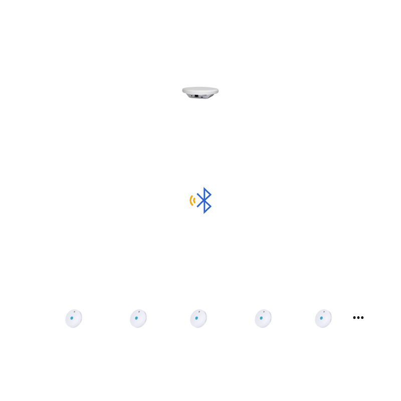
Deploying hundreds of BLE tags across a warehouse is the easy part. The hard part is making sure your gateways actually see them — consistently, at scale, without burning through scan windows that catch nothing but noise. This article breaks down the scanning side of the equation: how scan window and interval interact with tag advertising behavior, how to calculate detection probability, and how to tune gateway parameters for real-world deployment density.
1. Why Scanning Strategy Determines Project Success
A BLE tag broadcasting at 100 ms intervals is useless if the gateway’s scanner is asleep during those transmissions. Unlike continuous-stream protocols (WiFi, classic Bluetooth), BLE advertising is a one-shot, unidirectional burst. The scanner must be actively listening on the same advertising channel at the exact moment the tag transmits — otherwise the packet is gone forever.
Three factors determine whether a tag advertisement is captured:
| Factor | Controlled By | Typical Range |
|---|---|---|
| Advertising interval | Tag firmware | 20 ms – 1024 ms |
| Scan window / interval | Gateway scanner | 10 ms – 4096 ms |
| Advertising channel used | Tag (37/38/39, rotating) | 3 channels |
The detection probability is a function of all three. Getting it wrong means either missed detections (too-low duty cycle) or wasted gateway power and channel congestion (too-high duty cycle with diminishing returns).
2. BLE Scanning Fundamentals
2.1 Scan Window and Scan Interval
The BLE scanner operates with two key parameters:
– Scan Interval (T_scan): The period of one complete scan cycle. The scanner wakes up, listens for the scan window, then sleeps until the next cycle.
– Scan Window (T_window): The duration within each scan interval that the radio is actively receiving.
The scan duty cycle is:
Duty Cycle = T_window / T_scanA 120 ms scan window with a 1000 ms scan interval gives a 12% duty cycle. The scanner is listening 12% of the time.
2.2 Channel Scanning Behavior
BLE advertising uses three channels (37, 38, 39). During each scan window, the scanner listens on one channel — it rotates channels across scan intervals per the BLE specification. This means:
– A tag advertising on channel 37 will only be heard when the scanner happens to be listening on channel 37.
– With three channels, the scanner spends roughly 1/3 of its active time on each channel.
This is critical: a 12% duty cycle means only ~4% effective listening time per channel.
3. Detection Probability Model
3.1 The Basic Model
For a tag with advertising interval T_adv and a scanner with scan window T_window and scan interval T_scan, the probability of detecting at least one advertisement within one scan interval is:
P_detect = 1 - (1 - T_window / T_scan)^nWhere n = number of advertisements that occur during one scan interval:
n = T_scan / T_advSubstituting:
P_detect = 1 - (1 - T_window / T_scan)^(T_scan / T_adv)3.2 Worked Example
Consider a tag advertising every 500 ms, a scanner with 120 ms window and 1000 ms interval:
n = 1000 / 500 = 2 advertisements per scan interval
P_detect = 1 - (1 - 0.12)^2 = 1 - 0.7744 = 0.2256 (22.6%)
That is a 77.4% miss rate per scan interval. Over 10 scan intervals (10 seconds):
P_detect_10 = 1 - (1 - 0.2256)^10 = 1 - 0.0635 = 0.9365 (93.7%)So within 10 seconds, there’s a 93.7% chance of at least one detection. Whether that’s acceptable depends on your application’s latency requirement.
3.3 Channel Overhead Correction
Since the scanner only listens on one of three channels per interval, the effective detection probability drops further. The tag rotates across all three channels, and the scanner rotates independently. The probability that both are on the same channel is approximately 1/3 per advertisement.
Corrected model:
P_detect_corrected = 1 - (1 - T_window / (3 * T_scan))^(T_scan / T_adv)Re-running the example:
P_detect_corrected = 1 - (1 - 0.04)^2 = 1 - 0.9216 = 0.0784 (7.8%)Over 10 seconds (10 intervals):
P_detect_10_corrected = 1 - (1 - 0.0784)^10 = 1 - 0.4355 = 0.5645 (56.5%)That 56.5% detection rate over 10 seconds is far less reassuring. This is why naive parameter choices lead to “intermittent” tags in production.
4. Scan Parameter Optimization
4.1 Target Detection Latency Approach
Instead of guessing parameters, start with a target: “I want 99% detection within N seconds.” Then solve backwards.
For 99% detection within 10 seconds with a 500 ms advertising tag:
P_per_interval = 1 - (1 - 0.99)^(1/10) = 0.369
Solving: T_window / (3 * T_scan) >= 0.369 * (T_adv / T_scan)
With T_scan = 1000 ms, T_adv = 500 ms:
T_window >= 0.369 * 500 * 3 = 553.5 msA 554 ms scan window in a 1000 ms interval (55.4% duty cycle) achieves 99% detection within 10 seconds. That’s aggressive — and it illustrates the tradeoff: high detection rates demand high duty cycles.
4.2 Practical Parameter Matrix
The table below shows detection rates for common parameter combinations, assuming a 500 ms advertising interval with channel correction:
| Scan Window | Scan Interval | Duty Cycle | P(1 interval) | P(10s) | P(30s) |
|---|---|---|---|---|---|
| 60 ms | 1000 ms | 6% | 3.9% | 33.0% | 69.5% |
| 120 ms | 1000 ms | 12% | 7.8% | 56.5% | 91.4% |
| 250 ms | 1000 ms | 25% | 15.4% | 80.3% | 99.2% |
| 500 ms | 1000 ms | 50% | 28.0% | 95.7% | 99.98% |
| 1000 ms | 1000 ms | 100% | 48.8% | 99.6% | ~100% |
| 120 ms | 500 ms | 24% | 15.4% | 80.3% | 99.2% |
| 250 ms | 500 ms | 50% | 28.0% | 95.7% | 99.98% |
Key takeaways:
– Continuous scanning (100% duty cycle) still only yields ~49% per-interval detection due to channel rotation — but over 30 seconds it converges to ~100%.
– Doubling the scan window roughly doubles per-interval detection probability.
– Halving the scan interval has the same effect as doubling the window, but with different power implications.
4.3 Gateway Power Budget
Scanner power consumption is roughly linear with duty cycle. A gateway drawing 60 mA while actively scanning and 5 mA while idle:
| Duty Cycle | Avg Current | 24h Power (3.3V) |
|---|---|---|
| 12% | 11.8 mA | 935 mWh |
| 25% | 18.75 mA | 1485 mWh |
| 50% | 32.5 mA | 2574 mWh |
| 100% | 60 mA | 4752 mWh |
For mains-powered gateways, 100% duty cycle is viable. For battery-powered gateways (solar or primary cell), 12-25% is the practical ceiling.
5. Multi-Channel Scanning Strategies
5.1 Single-Radio Sequential Scanning (Default)
Standard BLE controllers cycle through channels 37→38→39 automatically. This is free — no firmware work needed — but the 1/3 effective duty cycle per channel is a fundamental limitation.
5.2 Pinned Channel Scanning
Some BLE stacks allow locking the scanner to a single channel (e.g., always listen on 37). If the tag is also configured to advertise only on channel 37, you eliminate the channel rotation penalty:
P_detect = 1 - (1 - T_window / T_scan)^(T_scan / T_adv)Using the earlier example (120 ms window, 1000 ms interval, 500 ms adv):
P_detect = 1 - (1 - 0.12)^2 = 0.2256 (22.6%)That’s 3x better than the 3-channel case (7.8%). The tradeoff: you lose redundancy. If channel 37 has persistent interference (e.g., from WiFi on channel 1), detection collapses entirely.
5.3 Dual-Radio Parallel Scanning
High-end gateways (e.g., ESP32 + nRF52 combo) can run two BLE radios simultaneously, each pinned to a different channel or running independent scan cycles. This doubles hardware cost but:
– Doubles effective scan coverage
– Enables concurrent active scanning on one radio and passive on another
– Allows one radio to handle connections while the other scans
With dual radios covering channels 37 and 38, and the tag advertising on all three:
P_detect = 1 - (1 - 2/3 * T_window / T_scan)^(T_scan / T_adv)This gives a 2/3 channel coverage factor instead of 1/3.
6. Active vs Passive Scanning
6.1 Passive Scanning
The gateway listens silently. It captures only advertising PDUs (ADV_NONCONN_IND, ADV_IND without response). This is the standard mode for asset tracking with BLE tags that broadcast iBeacon or Eddystone frames.
– Pros: Minimal gateway radio time per advertisement, no upstream interference
– Cons: No payload beyond the advertising packet (max 31 bytes)
6.2 Active Scanning
The gateway sends SCAN_REQ after receiving an advertisement. The tag responds with SCAN_RSP (another 31 bytes). This doubles the payload capacity to 62 bytes.
– Pros: Full manufacturer-specific data, sensor values in scan response
– Cons: Adds 150-200 μs per scan response, increases channel airtime, can cause collisions in dense tag deployments
6.3 Density Threshold
In a deployment with N tags advertising at interval T_adv on a single channel, the channel occupancy is:
Occupancy = N * (T_adv_pdu + T_scan_req_rsp) / T_advWhere T_adv_pdu ≈ 376 μs (37 bytes at 1 Mbps) and T_scan_req_rsp ≈ 376 μs (request + response).
For passive scanning (no scan response), occupancy with 200 tags at 1s interval:
Occupancy = 200 * 0.376ms / 1000ms = 7.5%For active scanning:
Occupancy = 200 * 0.752ms / 1000ms = 15.0%At 15% occupancy, collision probability becomes non-trivial. Above 30% (roughly 400 tags with active scanning at 1s), the collision rate degrades detection faster than scanning can compensate.
7. Gateway Placement and Density Planning
7.1 Coverage Overlap
Each gateway has a finite effective range, determined by tag TX power, antenna gain, and environmental attenuation. In a typical warehouse (15 m ceiling, metal racking):
| Tag TX Power | Practical Range | Tags per Gateway (1000 m² floor) |
|---|---|---|
| +4 dBm | 15-20 m | ~200-300 |
| 0 dBm | 10-15 m | ~100-200 |
| -12 dBm | 5-8 m | ~50-80 |
7.2 Gateway Density Formula
For a target detection latency of T_target seconds and tag count N with advertising interval T_adv:
Gateways = ceil(N * T_scan_window / (T_target * T_adv * P_threshold))Where P_threshold is the required per-interval detection probability. This is simplified — real planning also accounts for spatial distribution and RF propagation.
7.3 Practical Deployment Rule
For 95% detection within 10 seconds at 500 ms advertising interval:
– Open office: 1 gateway per 400 m², 25% scan duty cycle
– Warehouse with racking: 1 gateway per 250 m², 50% scan duty cycle
– Mixed environment (walls, machinery): 1 gateway per 150 m², 50% scan duty cycle
These assume +4 dBm tag TX power and standard dipole antennas on both ends.
8. Real-World Detection Rate Benchmarks
The following benchmarks were measured in a 2000 m² warehouse with 100 BLE tags (500 ms adv interval, +4 dBm TX power), 8 gateways (ESP32, 120 ms window, 500 ms interval, 24% duty cycle):
| Metric | Value | Notes |
|---|---|---|
| Avg detections per tag per minute | 8.3 | Expected: ~12 (24% duty cycle, 500 ms adv) |
| Tags with <95% detection rate | 7/100 | All in rack shadow zones |
| Tags with <80% detection rate | 2/100 | Behind metallic enclosures |
| Avg RSSI of detected packets | -67 dBm | Range: -45 to -89 dBm |
| Scan channel collision rate | 3.2% | From 8 overlapping gateways |
After tuning (increased duty cycle to 50%, added 2 gateways in shadow zones):
| Metric | Before | After |
|---|---|---|
| Tags with <95% detection | 7 | 1 |
| Tags with <80% detection | 2 | 0 |
| Avg detections per tag/min | 8.3 | 14.7 |
| Gateway power consumption | 18.7 mA avg | 32.5 mA avg |
The improvement cost: 73% more gateway power and 25% more hardware. Whether that tradeoff is justified depends on the cost of a missed detection in the specific application.
9. Summary and Recommendations
| Scenario | Scan Window | Scan Interval | Duty Cycle | Expected P(95% in 10s) |
|---|---|---|---|---|
| Mains-powered, dense tags | 500 ms | 1000 ms | 50% | ~96% |
| Mains-powered, sparse tags | 250 ms | 1000 ms | 25% | ~80% |
| Battery gateway, dense tags | 250 ms | 500 ms | 50% | ~96% |
| Battery gateway, sparse tags | 120 ms | 1000 ms | 12% | ~57% |
| Ultra-low-power gateway | 60 ms | 2000 ms | 3% | ~15% |
Rules of thumb:
1. Start with the tag advertising interval — it’s usually fixed by the tag’s power budget. Build the scanning strategy around it.
2. Target 50% duty cycle for production deployments — it’s the knee of the curve where detection probability rises sharply without excessive power cost.
3. Account for channel rotation — your effective per-channel duty cycle is 1/3 of the raw number. This is the most commonly missed factor in scanning design.
4. Benchmark in the actual environment — RF propagation in warehouses and factories is too variable for pure theoretical models. Deploy a few gateways, measure detection rates, then scale.
5. Consider pinned-channel scanning for controlled environments where you control both tag and gateway firmware. The 3x detection improvement is worth the loss of channel diversity in most indoor settings.